mst: Minimum Spanning Tree of the Pairwise Distance Graph

Description

Determine a(*) minimum spanning tree (MST) of the complete undirected graph representing a set of \(n\) points whose weights correspond to the pairwise distances between the points.

Usage

mst(d, ...)

## Default S3 method:
mst(
  d,
  distance = c("euclidean", "l2", "manhattan", "cityblock", "l1", "cosine"),
  M = 1L,
  verbose = FALSE,
  ...
)

## S3 method for class 'dist'
mst(d, M = 1L, verbose = FALSE, ...)

Arguments

d	either a numeric matrix (or an object coercible to one, e.g., a data frame with numeric-like columns) or an object of class dist; see dist
...	further arguments passed to or from other methods, in particular, to mst_euclid from the quitefastmst package
distance	metric used in the case where d is a matrix; one of: "euclidean" (synonym: "l2"), "manhattan" (a.k.a. "l1" and "cityblock"), "cosine"
M	smoothing factor; M = 1 selects the requested distance; otherwise, the corresponding degree-M mutual reachability distance is used; M should be rather small, say, \(\leq 20\)
verbose	logical; whether to print diagnostic messages and progress information

Details

(*) Note that if the distances are non unique, there might be multiple minimum trees spanning a given graph.

If d is a matrix and the use of Euclidean distance is requested (the default), then mst_euclid is called to determine the MST. It is quite fast in spaces of low intrinsic dimensionality, even for 10M points.

Otherwise, a much slower implementation of the Jarník (Prim/Dijkstra)-like method, which requires \(O(n^2)\) time, is used. The algorithm is parallelised; the number of threads is determined by the OMP_NUM_THREADS environment variable. As a rule of thumb, datasets up to 100k points should be processed relatively quickly.

If \(M>1\), then the mutual reachability distance \(m(i,j)\) with the smoothing factor \(M\) (see Campello et al. 2013) is used instead of the chosen “raw” distance \(d(i,j)\). It holds \(m(i, j)=\max\{d(i,j), c(i), c(j)\}\), where \(c(i)\) is the core distance, i.e., the distance between the \(i\)-th point and its (M-1)-th nearest neighbour. This makes “noise” and “boundary” points being “pulled away” from each other. The Genie clustering algorithm (see gclust) with respect to the mutual reachability distance can mark some observations as noise points.

Value

Returns a numeric matrix of class mst with \(n-1\) rows and three columns: from, to, and dist sorted nondecreasingly. Its i-th row specifies the i-th edge of the MST which is incident to the vertices from[i] and to[i] with from[i] < to[i] (in 1,…,n) and dist[i] gives the corresponding weight, i.e., the distance between the point pair.

The Size attribute specifies the number of points, \(n\). The Labels attribute gives the labels of the input points, if available. The method attribute provides the name of the distance function used.

If \(M>1\), the nn.index attribute gives the indices of the M-1 nearest neighbours of each point and nn.dist provides the corresponding distances, both in the form of an \(n\) by \(M-1\) matrix.

Author(s)

Marek Gagolewski and other contributors

References

V. Jarník, O jistem problemu minimalnim, Prace Moravske Prirodovedecke Spolecnosti 6, 1930, 57-63.

C.F. Olson, Parallel algorithms for hierarchical clustering, Parallel Computing 21, 1995, 1313-1325.

R. Prim, Shortest connection networks and some generalisations, The Bell System Technical Journal 36(6), 1957, 1389-1401.

O. Borůvka, O jistém problému minimálním, Práce Moravské Přírodovědecké Společnosti 3, 1926, 37–58.

J.L. Bentley, Multidimensional binary search trees used for associative searching, Communications of the ACM 18(9), 509–517, 1975, doi:10.1145/361002.361007. W.B. March, R. Parikshit, A.G. Gray, Fast Euclidean minimum spanning tree: Algorithm, analysis, and applications, Proc. 16th ACM SIGKDD Intl. Conf. Knowledge Discovery and Data Mining (KDD ‘10), 2010, 603–612.

R.J.G.B. Campello, D. Moulavi, J. Sander, Density-based clustering based on hierarchical density estimates, Lecture Notes in Computer Science 7819, 2013, 160-172, doi:10.1007/978-3-642-37456-2_14.

See Also

The official online manual of genieclust at https://genieclust.gagolewski.com/

Gagolewski, M., genieclust: Fast and robust hierarchical clustering, SoftwareX 15:100722, 2021, doi:10.1016/j.softx.2021.100722

mst_euclid

Examples

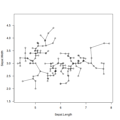
library("datasets")
data("iris")
X <- jitter(as.matrix(iris[1:2]))  # some data
T <- mst(X)
plot(X, asp=1, las=1)
segments(X[T[, 1], 1], X[T[, 1], 2],
         X[T[, 2], 1], X[T[, 2], 2])