gclust: Hierarchical Clustering Algorithm Genie

Description

A reimplementation of Genie - a robust and outlier resistant clustering algorithm by Gagolewski, Bartoszuk, and Cena (2016). The Genie algorithm is based on the minimum spanning tree (MST) of the pairwise distance graph of a given point set. Just like the Single Linkage method, it consumes the edges of the MST in an increasing order of weights. However, it prevents the formation of clusters of highly imbalanced sizes; once the Gini index (see gini_index()) of the cluster size distribution raises above gini_threshold, merging a point group of the smallest size is enforced.

A clustering can also be computed with respect to the \(M\)-mutual reachability distance (based, e.g., on the Euclidean metric), which is used in the definition of the HDBSCAN* algorithm (see mst() for the definition). For the smoothing factor \(M>0\), outliers are pulled away from their neighbours. This way, the Genie algorithm gives an alternative to the HDBSCAN* algorithm (Campello et al., 2013) that is able to detect a predefined number of clusters and indicate outliers (via deadwood; see Gagolewski, 2026) without depending on DBSCAN*’s eps or HDBSCAN*’s min_cluster_size parameters. Also make sure to check out the Lumbermark algorithm (package lumbermark) that is also based on MSTs.

Usage

gclust(d, ...)

## Default S3 method:
gclust(
  d,
  gini_threshold = 0.3,
  M = 0L,
  distance = c("euclidean", "l2", "manhattan", "cityblock", "l1", "cosine"),
  verbose = FALSE,
  ...
)

## S3 method for class 'dist'
gclust(d, gini_threshold = 0.3, M = 0L, verbose = FALSE, ...)

## S3 method for class 'mst'
gclust(d, gini_threshold = 0.3, verbose = FALSE, ...)

genie(d, ...)

## Default S3 method:
genie(
  d,
  k,
  gini_threshold = 0.3,
  M = 0L,
  distance = c("euclidean", "l2", "manhattan", "cityblock", "l1", "cosine"),
  verbose = FALSE,
  ...
)

## S3 method for class 'dist'
genie(d, k, gini_threshold = 0.3, M = 0L, verbose = FALSE, ...)

## S3 method for class 'mst'
genie(d, k, gini_threshold = 0.3, verbose = FALSE, ...)

Arguments

d	a numeric matrix (or an object coercible to one, e.g., a data frame with numeric-like columns) or an object of class dist (see dist), or an object of class mst (see mst)
...	further arguments passed to mst()
gini_threshold	threshold for the Genie correction, i.e., the Gini index of the cluster size distribution; threshold of 1.0 leads to the single linkage algorithm; low thresholds highly penalise the formation of small clusters
M	smoothing factor; \(M \leq 1\) gives the selected distance; otherwise, the mutual reachability distance is used
distance	metric used to compute the linkage, one of: "euclidean" (synonym: "l2"), "manhattan" (a.k.a. "l1" and "cityblock"), "cosine"
verbose	logical; whether to print diagnostic messages and progress information
k	the desired number of clusters to detect

Details

As with all distance-based methods (this includes k-means and DBSCAN as well), applying data preprocessing and feature engineering techniques (e.g., feature scaling, feature selection, dimensionality reduction) might lead to more meaningful results.

If d is a numeric matrix or an object of class dist, mst() will be called to compute an MST, which generally takes at most \(O(n^2)\) time. However, by default, a faster algorithm based on K-d trees is selected automatically for low-dimensional Euclidean spaces; see mst_euclid from the quitefastmst package.

Once a minimum spanning tree is determined, the Genie algorithm runs in \(O(n \sqrt{n})\) time. If you want to test different gini_thresholds or \(k\)s, it is best to compute the MST explicitly beforehand.

Due to Genie’s original definition, the resulting partition tree (dendrogram) might violate the ultrametricity property (merges might occur at levels that are not increasing w.r.t. a between-cluster distance). gclust() automatically corrects departures from ultrametricity by applying height = rev(cummin(rev(height))).

Value

gclust() computes the entire clustering hierarchy; it returns a list of class hclust; see hclust. Use cutree to obtain an arbitrary \(k\)-partition.

genie() returns an object of class mstclust, which defines a \(k\)-partition, i.e., a vector whose \(i\)-th element denotes the \(i\)-th input point’s cluster label between 1 and \(k\).

In both cases, the mst attribute gives the computed minimum spanning tree which can be reused in further calls to the functions from genieclust, lumbermark, and deadwood. For genie(), the cut_edges attribute gives the \(k-1\) indexes of the MST edges whose omission leads to the requested \(k\)-partition (connected components of the resulting spanning forest). In gclust(), these are exactly the last \(k-1\) indexes in the links attribute (but sorted).

Author(s)

Marek Gagolewski and other contributors

References

M. Gagolewski, M. Bartoszuk, A. Cena, Genie: A new, fast, and outlier-resistant hierarchical clustering algorithm, Information Sciences 363, 2016, 8-23, doi:10.1016/j.ins.2016.05.003

R.J.G.B. Campello, D. Moulavi, J. Sander, Density-based clustering based on hierarchical density estimates, Lecture Notes in Computer Science 7819, 2013, 160-172, doi:10.1007/978-3-642-37456-2_14

M. Gagolewski, A. Cena, M. Bartoszuk, Ł. Brzozowski, Clustering with minimum spanning trees: How good can it be?, Journal of Classification 42, 2025, 90-112, doi:10.1007/s00357-024-09483-1

M. Gagolewski, genieclust: Fast and robust hierarchical clustering, SoftwareX 15, 2021, 100722, doi:10.1016/j.softx.2021.100722

M. Gagolewski, deadwood, in preparation, 2026

M. Gagolewski, quitefastmst, in preparation, 2026

See Also

The official online manual of genieclust at https://genieclust.gagolewski.com/

Gagolewski, M., genieclust: Fast and robust hierarchical clustering, SoftwareX 15:100722, 2021, doi:10.1016/j.softx.2021.100722

mst() for the minimum spanning tree routines

normalized_clustering_accuracy() (amongst others) for external cluster validity measures

Examples

library("datasets")
data("iris")
X <- jitter(as.matrix(iris[3:4]))
h <- gclust(X)
y_pred <- cutree(h, 3)
y_test <- as.integer(iris[,5])
plot(X, col=y_pred, pch=y_test, asp=1, las=1)

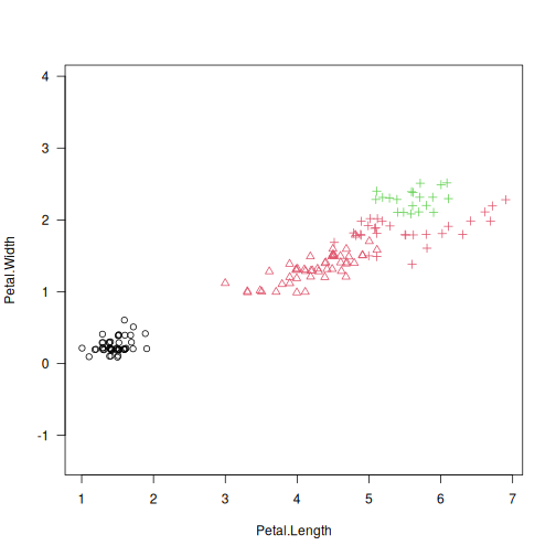
adjusted_rand_score(y_test, y_pred)
## [1] 0.5993085
normalized_clustering_accuracy(y_test, y_pred)
## [1] 0.7
# detect 3 clusters and find outliers with Deadwood
library("deadwood")
y_pred2 <- genie(X, k=3, M=5)  # the 5-mutual reachability distance
plot(X, col=y_pred2, asp=1, las=1)
is_outlier <- deadwood(y_pred2)
points(X[!is_outlier, ], col=y_pred2[!is_outlier], pch=16)