Outlier Detection with Deadwood¶

The Deadwood outlier detection algorithm[1] can be run on the clustered dataset to identify anomalous points in each cluster. This may be beneficial where the clusters are of heterogeneous densities.

import numpy as np
import pandas as pd
import matplotlib.pyplot as plt
import genieclust
import deadwood

def plot_scatter(X, labels=None):
    deadwood.plot_scatter(X, labels=labels, asp=1, alpha=0.5, markers='o', s=10)

Let’s load an example dataset that can be found at the hdbscan [14] package’s project site:

dataset = "hdbscan"
X = np.loadtxt("%s.data.gz" % dataset, ndmin=2)
labels_true = np.loadtxt("%s.labels0.gz" % dataset, dtype=np.intp) - 1
n_clusters = len(np.unique(labels_true[labels_true>=0]))

Here are the reference labels as identified by a manual annotator. The light gray markers corresponding to the label -1 designate outliers.

plot_scatter(X, labels_true)
plt.title("(n=%d, true n_clusters=%d)" % (X.shape[0], n_clusters))
plt.axis("equal")
plt.show()

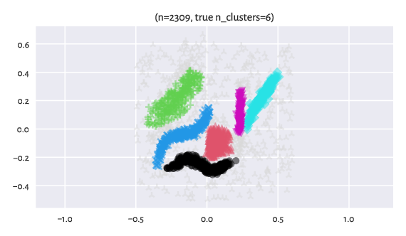
../_images/noise-scatter-1.png — Figure 10 Reference labels¶

Smoothing Factor¶

The genieclust package allows for clustering with respect to the mutual reachability distance, \(d_M\), known from the DBSCAN* algorithm [2]. This metric is parameterised by a smoothing factor, \(M\ge 1\).

Namely, instead of the ordinary (usually Euclidean) distance between two points \(i\) and \(j\), \(d(i,j)\), we take \(d_M(i,j)=\max\{ c_M(i), c_M(j), d(i, j) \}\), where the so-called \(M\)-core distance \(c_M(i)\) is the distance between \(i\) and its \(M\)-th nearest neighbour (here, not including \(i\) itself, unlike in [2]).

DBSCAN* and its hierarchical version, HDBSCAN*, introduces the notion of noise and core points. Furthermore, their predecessor, DBSCAN, also marks certain non-core values as border points. They all rely on a specific threshold \(\varepsilon\) that is applied onto the points’ core distances.

In our case, we can perform anomaly detection on subsets of mutual reachability minium spanning trees using the Deadwood algorithm, separately in each cluster identified by Genie.

Here are the effects of playing with the \(M\) parameter (we keep the default gini_threshold):

Ms = [10, 25]
for i in range(len(Ms)):
    g = genieclust.Genie(n_clusters=n_clusters, M=Ms[i]).fit(X)
    labels = g.labels_.copy()
    d = deadwood.Deadwood().fit(g)
    labels[d.labels_ < 0] = -1
    plt.subplot(1, 2, i+1)
    plot_scatter(X, labels)
    plt.title("(gini_threshold=%g, M=%d)"%(g.gini_threshold, g.M))
    plt.axis("equal")
plt.show()

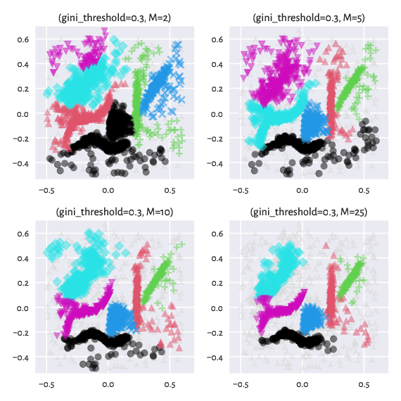
../_images/noise-Genie1-3.png — Figure 11 Labels predicted by Genie with outliers detected by Deadwood¶

Cluster Hierarchy¶

Contrary to the HDBSCAN* method featured in the hdbscan package [14], in our case, we can request a specific number of clusters. Moreover, we can easily switch between partitions of finer or coarser granularity. Genie is a hierarchical algorithm, so the partitions are properly nested.

ncs = [3, 6, 8, 10]
for i in range(len(ncs)):
    g = genieclust.Genie(n_clusters=ncs[i], M=10).fit(X)
    labels = g.labels_.copy()
    d = deadwood.Deadwood().fit(g)
    labels[d.labels_ < 0] = -1
    plt.subplot(2, 2, i+1)
    plot_scatter(X, labels)
    plt.title("(n_clusters=%d)"%(g.n_clusters))
    plt.axis("equal")
plt.show()

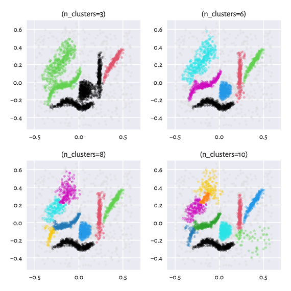
../_images/noise-Genie3-5.png — Figure 12 Labels predicted by Genie with outliers removed by Deadwood: Different number of clusters requested¶

A Comparision with HDBSCAN*¶

Here are the results returned by hdbscan with default parameters:

import hdbscan
h = hdbscan.HDBSCAN()
labels_hdbscan = h.fit_predict(X)
plot_scatter(X, labels_hdbscan)
plt.title("(min_cluster_size=%d, min_samples=%d)" % (
    h.min_cluster_size, h.min_samples or h.min_cluster_size))
plt.axis("equal")
plt.show()

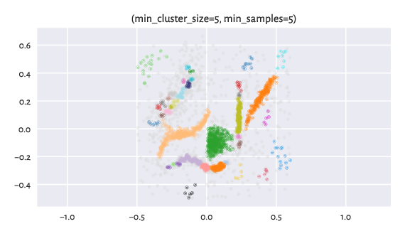
../_images/noise-HDBSCAN1-7.png — Figure 13 Labels predicted by HDBSCAN*.¶

By tuning up min_cluster_size and/or min_samples (which corresponds to our M; min_samples defaults to min_cluster_size if not provided explicitly), we can obtain a partition that is even closer to the reference one:

mcss = [10, 25]
mss = [10, 25]
for i in range(len(mcss)):
    for j in range(len(mss)):
        h = hdbscan.HDBSCAN(min_cluster_size=mcss[i], min_samples=mss[j])
        labels_hdbscan = h.fit_predict(X)
        plt.subplot(len(mcss), len(mss), i*len(mss)+j+1)
        plot_scatter(X, labels_hdbscan)
        plt.title("(min_cluster_size=%d, min_samples=%d)" % (
            h.min_cluster_size, h.min_samples or h.min_cluster_size))
        plt.axis("equal")
plt.show()

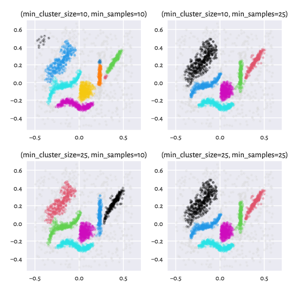
../_images/noise-HDBSCAN2-9.png — Figure 14 Labels predicted by HDBSCAN* – different settings¶