Basic Usage (R)

The latest stable release of the R package genieclust is available from the CRAN repository. Install it by calling:

install.packages("genieclust")

Below are a few basic examples of interacting with the package.

library("genieclust")

Let’s take the Sustainable Society Indices dataset that measures the Human, Environmental, and Economic Wellbeing in each country. There are seven categories on the scale \([0, 10]\).

# see https://github.com/gagolews/genieclust/tree/master/devel/sphinx/weave
ssi <- read.csv("ssi_2016_categories.csv", comment.char="#")
X <- as.matrix(ssi[,-1])    # everything except the Country (1st) column
dimnames(X)[[1]] <- ssi[,1] # set row names
head(X)  # preview
##           BasicNeeds PersonalDevelopmentAndHealth WellBalancedSociety
## Albania       9.6058                       7.9596              6.9926
## Algeria       9.0212                       7.3365              4.2039
## Angola        5.9728                       5.6928              2.1401
## Argentina     9.8320                       8.3506              3.8952
## Armenia       9.4469                       7.4205              6.2892
## Australia    10.0000                       8.5909              6.1055
##           NaturalResources ClimateAndEnergy Transition Economy
## Albania             6.6343           4.6217     2.1025  3.0565
## Algeria             5.2772           2.6627     3.0741  6.1543
## Angola              6.7594           6.2122     1.8988  3.7535
## Argentina           5.4535           3.3003     6.3899  5.3406
## Armenia             6.4363           2.8543     2.4342  3.8296
## Australia           4.1307           1.6278     7.5395  7.5931

The API of genieclust is compatible with R’s workhorse for hierarchical clustering, stats::hclust(), which accepts a complete pairwise distance matrix. Yet, for better performance, it is better to feed genieclust::gclust() with the input data matrix directly:

# faster than gclust(dist(X)):
h <- gclust(X)  # default: gini_threshold=0.3, distance="euclidean"
print(h)
## 
## Call:
## gclust.mst(d = tree, gini_threshold = gini_threshold, verbose = verbose)
## 
## Cluster method   : Genie(0.3) 
## Distance         : euclidean 
## Number of objects: 154

In order to extract a desired k-partition, we can call stats::cutree():

y_pred <- cutree(h, k=3)  # also: genie(X, 3)
sample(y_pred, 25)  # preview
##                Iran            Slovenia             Morocco 
##                   1                   3                   1 
## Trinidad and Tobago        Sierra Leone            Colombia 
##                   1                   2                   1 
##        Turkmenistan               Syria             Nigeria 
##                   1                   1                   2 
##             Tunisia               Ghana              Sweden 
##                   1                   2                   1 
##         Netherlands              Bhutan              Mexico 
##                   3                   1                   1 
##             Jamaica        Saudi Arabia             Hungary 
##                   1                   1                   3 
##                Peru          Kazakhstan               Spain 
##                   1                   1                   3 
##               Japan        Korea, North               China 
##                   1                   1                   1 
##             Liberia 
##                   2

This gives the cluster IDs allocated to each country.

Note

If we are only interested in the partition of a specific cardinality, calling genie() directly will be slightly faster than referring to cutree(gclust(...)).

Let’s depict the obtained partition using the rworldmap package:

library("rworldmap")  # see the package's manual for details
mapdata <- data.frame(Country=dimnames(X)[[1]], Cluster=y_pred)
mapdata <- joinCountryData2Map(mapdata, joinCode="NAME", nameJoinColumn="Country")
mapCountryData(mapdata, nameColumnToPlot="Cluster", catMethod="categorical",
    missingCountryCol="white", colourPalette=palette.colors(3, "R4"),
    mapTitle="")

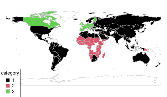
Figure 15 Countries grouped with respect to the SSI categories

We can compute, for instance, the average indicators in each identified group:

t(aggregate(as.data.frame(X), list(Cluster=y_pred), mean))[-1, ]
##                                [,1]   [,2]   [,3]
## BasicNeeds                   9.0679 5.2689 9.8178
## PersonalDevelopmentAndHealth 7.5081 5.9312 8.2995
## WellBalancedSociety          4.8869 2.8682 6.8272
## NaturalResources             5.6633 7.0040 6.3743
## ClimateAndEnergy             3.6241 7.0818 3.5947
## Transition                   4.0749 2.6300 7.3402
## Economy                      5.5127 3.5411 4.2742

Dendrograms

Dendrogram plotting is also possible. For better readability, we will restrict ourselves to a smaller sample; namely, to the 37 members of the OECD:

oecd <- c("Australia", "Austria", "Belgium", "Canada", "Chile", "Colombia",
"Czech Republic", "Denmark", "Estonia", "Finland", "France", "Germany",
"Greece", "Hungary", "Iceland", "Ireland", "Israel", "Italy", "Japan",
"Korea, South", "Latvia", "Lithuania", "Luxembourg", "Mexico", "Netherlands",
"New Zealand", "Norway", "Poland", "Portugal", "Slovak Republic", "Slovenia",
"Spain", "Sweden", "Switzerland", "Turkey", "United Kingdom", "United States")
X_oecd <- X[dimnames(X)[[1]] %in% oecd, ]
h_oecd <- gclust(X_oecd)
plot(as.dendrogram(h_oecd), horiz=TRUE)

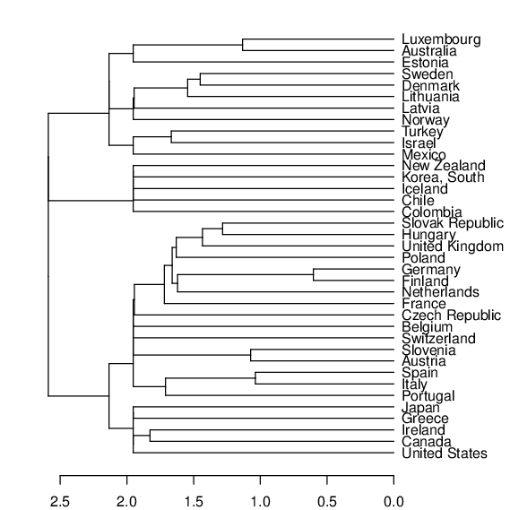
Figure 16 Cluster dendrogram for the OECD countries

Outlier Detection with Deadwood

The Deadwood outlier detection algorithm can be run on the clustered dataset to identify anomalous points in each cluster. See the deadwood package tutorials for more details.

Remarks

genieclust also features partition similarity scores (such as the adjusted Rand index) and internal cluster validity measures (e.g., the Caliński-Harabasz index).

For more details, refer to the package’s documentation.

To learn more about R, check out Marek’s open-access textbook Deep R Programming [6].